Supply and Demand: The Market Mechanism
Price provides the incentive to both the consumer and producer. High prices encouraged more production by the producers, but less consumption by the consumers. Low prices discourage production by the producer, and encouraged consumption by the consumers. Both incentives push the price to balance the forces of consumption (demand) and production (supply). Economists call this balance: equilibrium. This natural mechanism requires no external institution for direction (or only a minimum amount), or any altruists motivation by either the consumers or the producers.
The supply and demand mechanism (the economic model) besides being the natural consequences of economic forces provides the most efficient economic outcomes possible. Satisfaction for society is maximized, at minimum cost. The market mechanisms efficiency outcome is always located on the production possibility curves frontier, where all resources are fully utilized (points within the production possibility curves are inefficient by definition, since resources are not being utilized). This core model of supply and demand explains why economists usually favor market results, and seldom wishes to interfere with price. Setting minimum wages, for instance, or interfering with trade, violate the spirit of the model, and lead to inefficient outcomes.
Alternative Viewpoints
This disagreement among economist is a matter of degree. Even Adam Smith, the father of economic saw a role for government in the economy. Lassize faire (government stay out) was never seen as absolute. The Government was needed to provide some elements of the following; law and order, enforcement of private contracts and property rights, public goods such as roads and other public infrastructure, and defense from external military threats. Most economists believe these roles continue. Most economists also believe that the market is a useful tool and has a place in the economy. The real difference is the degree of faith in the efficiency of the market, and whether society should take direction from the market, or society should control and direct the market.
How
are prices set? (The supply and demand model)
If no single seller or buyer can set prices and neither does government or any other institution; how are goods and services allocated in competitive markets, and how are resources allocated in the competitive factor markets? The answer is that there are two independent factors that determine price in competitive markets (demand and supply). If markets were not competitive by definition a single seller or buyer could control and set price. Competition then needs flexible impersonal pricing. Suppliers must not work together to influence prices, and each supplier must be able to enter or exit a market at will. There are a number of other conditions necessary for full competition, but let's look, first at the two principle components of the model, starting with demand.
Demand
(Substitution and Income effects)
The investigation of the market mechanism starts with a single consumer. A consumer will respond to price. Demand is a set of relationships that show the quantity of a good the consumer will buy at each price within a specific time period. To have an effective demand a consumer must both desire the product and be able to afford the good or service. Desire without the ability to afford a good or service is not demand. Therefore not everyone can equally participate as consumers in all markets (it depends on their wealth).
When the price of some item that is normally purchased increases or decreases, the consumer will buy less or more of it. There are two reasons for this:
First, an increase in the price of something that the consumer wants to buy makes the consumer poorer. It will now require a larger portion of income to purchase the same amount that the consumer uses to buy at the lower price. This affect is referred to as income effect. Price changes always affect one's real income (price increases decrease real income while price decreases increase real income). Its importance, however, varies with how large the cost of the item is relative to the consumers total budget. The change in price of salt will have a minimal affect on real income, while a change in the price of a car can be significant.
Second, you respond to the price of an item in relationship to other items. This effect is called the substitution effect. As the price of a good falls (other prices remaining unchanged), the good becomes relatively cheaper than other goods and you substitute the good for others goods that are now relatively more expensive. As the price of a good rises, you substitute other now less expensive goods for the one in question.
In general these two effects reinforce each other, with higher prices reducing the quantity of demand, and lower prices increasing the quantity of demand. But there can be exceptions. A Veblen good appeals to customers because of its high price (and status). Russian caviar, large diamonds and large luxury cars or yachts may be examples. Raising the price for these goods may not decrease quantity demanded.
Nonprice influences on demand
These factors include; first, prices of other products, both complements and substitutes. Complements our products used in conjunction with the good in question (in the United States movie going, and popcorn consumption are complements). If the price of a complement goes up, the demand for the good in question will decrease (as well as the complement itself). Substitutes are goods that replace each other in consumption (chicken, beef, and pork are substitutes). If the price of a substitute goes up, the demand for the good in question will go up (while the demand for the substitute declines). Second, changes in consumers income will affect the consumer's ability to buy, and thus their demand. Third, is a catch all category, which includes the preferences of the consumers. Changes in preferences will affect demand. These changes in desire and taste are usually not addressed by economist as part of the economic model of demand and supply. Economists usually refer to sociologist, psychologist and other social sciences to model these changes. This category is nonetheless important for the efficiency arguments of the model. If economists really want to argue that the market produces just the right goods and services then they have to implicitly believe that demand is innate to humans (not easily influence by producers and our general environment). How preferences are really formed help determine who is, in fact, in charge of the markets. The critics (alternative models) believe that preferences are not innate, but preferences are learned and influenced by producers (by using marketing strategies).
Law of demand
Figure 1. Individual and Market Demand Curves
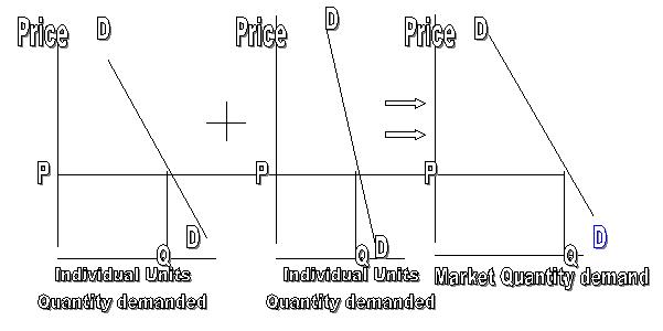
The demand curve shows an inverse relationship between price and quantity demanded. This relationship is considered so pervasive, particularly for the market demand, that in economics it has been termed the law of demand. The higher the price the lower the quantity demanded, and the lower the price the higher the quantity demanded. Although the law of demand is not logically absolutely necessary, given the case mentioned earlier of a Veblen luxury good, most goods or services are believed to adhere to the law of demand.
Price elasticity of demand
Inelastic demand would be expected for goods with the following characteristics; goods or services with no close substitutes, goods that are seen as necessities (not easily replaced), and goods that are inexpensive and a small part of a consumers budget. Also the shorter the time period of adjustment to a price change, the less elastic the market demand will be. For instance, gasoline is considered an inelastic good. A 20 percent increase in its price would not in the United States result in a 20 percent decrease in quantity demanded, the response would be much less. Gasoline has no close substitutes; gasoline (in much of the United States) is a necessity and has only a moderate affect on budgets (for the non-poor). In the short term, given the individuals cars gasoline requirements, and the distance between home, job, and school, there can be little adjustment of demand to gasoline price. Over a longer period of time new more efficient automobiles could be manufactured, mass transit could be developed, and distances traveled by consumers could be reduced (by moving closer to ones work or school etc.), which all would increase the elasticity of the gasoline market (but only as measured in the long term).
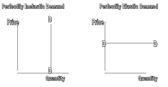
In figure 1 above, the middle graph shows a consumer less sensitive to price (the demand curve is closer to vertical), with a relatively inelastic demand, as compared to the more elastic demand of the consumer represented by the graph to the left. The value of the demand curves slope is not equal to its elasticity, since elasticity is defined as the percentage changes (but it's close for our purposes). In figure 2, perfectly elastic and inelastic cures are showed. Determining market elasticity is an empirically important process for understanding how markets work. In general markets work best when demand is elastic.
Figure 2, Inelastic and elastic demand curves
Shifting demand
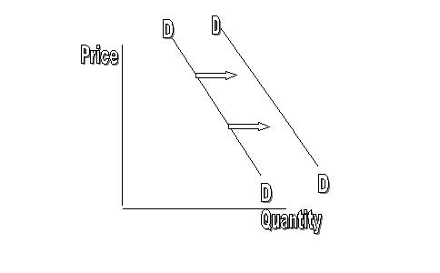
Figure 3, shows a hypothetical case for an increase in consumer income on the demand relationship. This good is considered a normal good because as income increases demand increases. An inferior good, in contrast, shows decrease demand as income increases (in this case the shift in the demand curve would be to the left). Examples of inferior goods in the United States might be the consumption of macaroni and cheese, or used cars.
Figure 3, Shifting demand curve
Supply
(the other half)
Supply is the relationship showing the quantities of a goods or services, that will be offered for sale at each price within a specific time period. The supply curve presupposes competition among firms so that no one firm can set and influence price. Firms are small relative to the market, and are price takers. Each small firm would provide a quantity of output for each possible price. Combining each firms quantity of output at each price for all firms provides a market supply relationship and thus a supply curve. Large firms (large relative to their market) such as monopolies and oligopolies set and influence price, and are not included in the supply curve, and in the analysis below. Because of their control of price, they can set their quantity of output to their advantage.
In contrast, to demand, the supply relationship shows a direct relationship between price and the quantity supplied. High prices encourage firms to produce more, while low prices discourage production. At high prices more resources can be used in production, and more firms with higher costs can find it profitable to produce. The reverse is true for low prices. This direct positive relationship between price and quantity supplied is called the law of supply.
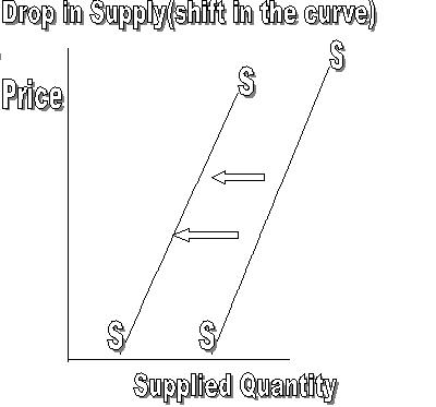
Change in quantity supplied verses change in supply
In contrast, a shift in the supply curve is a result of a number of outside variables (other than price) that change. The following are some of the more important outside variables.
First, improvements in technology which reduced costs and expand output make it possible for firms to offer more products for sale at each price. This may be particularly significant for certain technologically important market, such as communications and computer products.
Second, a reduction in price of inputs in the production process can allow firms to increase output at each and every price, while a increase in price of inputs reduce supply at each possible price.
Third, the prices and profitability of using resources in other alternative production processes can influence the firms production plans at each price level. For instance, if the firm suddenly has an opportunity to produce, with its resources, a new more profitable product, it may reduce the supply of other products.
Fourth, new firms may enter, while other firms may exit an industry. One of the important features of globalization is the large expansion in number of producers in the same enlarged worldwide market. There are other factors that cans shift a supply curve. For instance, for agricultural products weather conditions can dramatically affect the supply of a product. In the grain markets the variations in supply due to weather conditions has a long history of affecting price and the supply curve.
Implicit within the model of supply and demand is the underlying contention that price is the important variable, and not those external variables that shift the curves. The graphics of supply and demand use price on the vertical axes to represent the important causal variable. Many economic alternatives approaches imply with their analysis, that price is not necessarily this primary variable in all markets. One could argue, for instance, that in agricultural markets, and high-technology markets, that price, and adjustments to price are not the causal variable. Other variables that shift the curves, and help set price, and certainly influence price are the variables that need to be understood first to understand the industry and the changing market.
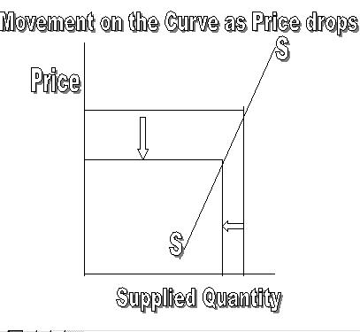
Unfortunately, in most markets in the real world it is difficult to determine, if there has been a shift in the curve, or a movement on the curve. The supply curve is only hypothetical. Empirically with only a price and quantity at one point in time, it is difficult to know what is causing what. Neoclassical economics generally assumes that markets are driven by price and is the primary causal variable.
Figure 4, Movement on the supply curve, and a shift in the supply curve
Elasticitys of supply
Grain markets usually suffer from inelastic supply conditions. To the extent that farming is seen as a way of life, and not a business, adjustment to prices is difficult, painful and slow. Grain prices that stay low, eventually have forced farmers off the land. This migration off the farm has been going on for centuries and still continues through the 20th century. But there are few alternative uses to farmland, so as farmers leave the land, farms only grow in size. But land still stays in cultivation. So grain supply may not change even with low prices, and once crops are planted each year, little can be done during the year to adjust to low prices. Grain output in the short term are not effected by price (resulting in an inelastic supply curve), but output is effected by weather conditions, which shift the supply curve.
The
market and equilibrium pricing
The market combines in exchange, both buyers and sellers. For economics it combines the demand and the supply curve to determine price. This price is called an equilibrium price, since it balances the two forces of supply and demand. An equilibrium price is the price at which the quantity demanded is equal to the quantity supplied. The quantity supplied and demanded is also referred to as the equilibrium quantity. Figure 5, shows both demand and supply determining equilibrium price and quantity.
Figure 5, Demand and supply and equilibrium
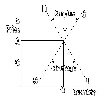
In figure 5, A is the equilibrium price and Q is the corresponding equilibrium quantity. At the price A the quantity supplied and a quantity demanded are equal, and at the Q quantity, demand and supply are equal.
If price were at B the quantity that suppliers would like to supply would be larger than consumers would demand at that price, creating a surplus quantity. A surplus would create forces among the many competitive suppliers to cut prices (supplier are all relatively small). Those forces would push the price down to the equilibrium level at A.
If prices were at C the quantity that suppliers would like to supply, would be less than consumers would demand at that price, creating a shortage. Because of the shortage and a competition among consumers, prices would tend to rise. Only at A would there be no tendency for the price to change, and A is the equilibrium price.
This graph represents the objective impersonal operation of the market. No one sets the price, and if the consumers dont like the price, they have no one to blame, and no recourse (over the price). If suppliers dont like the price, they in turn have no one to blame and no recourse (over the price). This is seen by many as one of the strength of markets.
Shifting demand and supply curves
Figure 6, Increase in demand and a decrease in supply
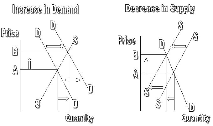
In figure 6, the first diagram on the left, shows an increase in demand with the new demand curve shifted to the right. This increase in demand with increased quantity demanded at each price could represent a case where income had increased, or where product desirability increased. As a result the equilibrium price has shifted from price level A to the higher price level B. The equilibrium quantity has also increased as new output has been brought onto the market as firms react to the higher prices. Therefore both prices and quantity has increased.
In figure 5, the second diagram on the right, shows a decrease in supply with a new supply curve shifted to the left. This decrease in supply (less quantity supplied at each price) could represent, poor weather in a crop growing area, or higher input prices due to shortages of crude oil, or labor. Price again has increased from the price level A to B, while quantity has declined as consumers react to the higher prices.
Not shown here are the other two cases where demand shifts to the left (decrease in demand), and where supply shift to the right (increase in supply). The logical consequences of these shifts are easily determined graphically. The difficulty in the real world is determining what actually has changed, and what has not, and by how much. In a dynamic changing market shifting curves, representing changing income, tastes, technical conditions, weather conditions and other variables might all overwhelm the forces pushing for equilibrium. In such an environment, equilibrium would never be reached, and the tools of supply and demand curves and its equilibrium analysis, would have minimum usefulness. To understand the market would require understanding how the institutions, technologies and those other outside variables are changing and evolving.
![]() Figure
7, demand and supply curve with no equilibrium possible.
Figure
7, demand and supply curve with no equilibrium possible.
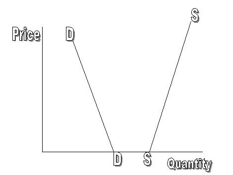
Figure 7, shows a case that is logically possible with no equilibrium price or quantity. Neither the law of supply or the law of demand is violated. Graphically if there was to be an equilibrium price it would have to be negative, which is impossible in the real world. Both demand and supply curves show a relatively inelastic relationship, where neither quantity demanded, or quantity supplied is sensitive to price. These markets operate poorly with a continuous oversupply, and thus a tendency for price to drop. Institutional factors (including government), depending on the consequences to the suppliers or customers, would keep the price above zero, but no conventional equilibrium would be possible.
Markets and their equilibrium price and quantity, function best with elastic demand and supply conditions. Here no outside intervention is likely with price providing enough incentive for both consumers and suppliers to reach equilibrium. Where price is important for both consumers and suppliers it is also unlikely that outside variables will overwhelm its impact. So in general markets function best when price is the focal point for both consumers and suppliers. There are many different markets where these price sensitivities differ among markets in both the long-term (many years) and over the short term.
Economic
efficiency and the market
In neoclassical economics the market has two distinct properties. The first, already discussed was the development of market equilibrium. Most mainstream economic models view the economy as sufficiently competitive, and as moving to equilibrium. This movement is seen as inevitable in the long haul, and as natural consequences of the economic forces of supply and demand. The movement to equilibrium is also seen as good because it is considered economically efficient. Although efficiency is not seen as the only criteria to judge the success of the economy, it does have in economics of special role and prominence. There is a belief among economists that economic theory can contribute to both an understanding of, and a promotion of economic efficiency.
There are other criteria for judging the success of an economy. The most prominent is equity or fairness. Fairness is seen as purely subjective. For economists, this criteria is seen as purely a judgment call, were economic theory has no role. Markets are not seen as particularly equitable or fair, they are just seen as objective phenomenon. And although fairness as criteria should be seen as potentially equal to efficiency, but because economists have little to add about fairness, fairness tends to be invisible in much of economic analysis.
The second, property of neoclassical economics is that markets are economically efficient. For economists, efficiency means that the economy is producing just the right quantity of goods and services to satisfy societys wants at minimum cost. Economic efficiency is not the engineering or technical definition of efficiency. Economic efficiency does not try only to minimize inputs in a production process, or even minimize costs in a given operation, or maximize output given a level of input, but determine for the whole economy what quantity of goods and services are best (given the demand curve), and minimize all opportunity costs for those goods and services.
Developing the full argument for economic efficiency in neoclassical economics requires a more complete development of demand and supply (perfect competition). These arguments are laid out more in the chapter on demand, and the chapter on perfect competition. But we can summarize the essence of those chapters on the meaning of demand and supply here. Given the assumptions of neoclassical economics on the theory of demand, the market demand curve is re-interpreted as the benefits to society (simply the addition of benefits to all individuals in society) in the consumption of goods and services. The demand curve represents the importance to society of these goods and services.
The other half of the efficiency equation comes from the supply curve. Here given the appropriate assumptions of perfect competition on the theory of supply, the market supply curve is re-interpreted as the cost to society for the consumption of goods and services. These are opportunity costs (that which has to be given up, to get something else) not necessarily only dollars. The supply curve represents the cost in production of goods and services.
Figure 8, shows the interpretation of supply and demand, as costs and benefits in the efficiency model. Economists measure these costs and benefits as marginal, (extra costs and extra benefits) on the curves.
Figure 8, Marginal cost and benefits in the efficiency model

In figure 8, an ordinary market demand and supply curve are shown. The graph on the left shows a demand curve with three quantity levels of demand. At the low quantity level A the relative benefit for the good is high resulting in a high price. Price measures the benefits of the extra unit (marginal) of this good and at low quantities (A) price is high. As quantity increases to B and then to C the benefit or price of another units declines (as shown on the graph). The common sense notion of this relationship is simply that as quantity increases saturation decreases the value of additional units. While total benefits (of all goods consumed) still increase the extra or marginal value of each additional unit declines.
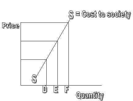
The graph on the right shows a supply curve with three quantity levels of supply. At the low quantity level D the social cost for producing the good is low per unit, resulting in a low price. Price for supply measures the cost of the extra unit (marginal) of this good and with low quantities (D) price is low. As quantity increases to E and then to F the social cost of supply, with additional units, increases (as shown on the graph). The notion is simply that all social costs escalate with increased output during a short period time, given limited capital resources (plant size and infrastructure is limited).
In figure 9, the efficiency model of neoclassical economics combines the demand curve or the benefits to consumption with the supply curve or the cost of that consumption.
Figure 9, Efficiency model
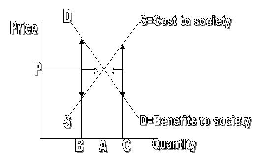
In graph 9, the equilibrium price is P with the corresponding equilibrium quantity as A. This result is seen as an automatic consequence of market behavior. The efficiency argument adds that these equilibrium results also are economically efficient. So that markets provided an efficient equilibrium outcome for society.
Quantity B is not efficient, because at quantity B the benefit to society for the good in question, is larger than the cost to society for its production. The line with arrows at B graphically represents this gap. If more quantity would be produced and consumed benefits would be expanded more than costs and there would be a net gain in value. The inefficiency would decrease as quantity increases and the gap disappears. At A there is no gap and the benefits to society of consuming another unit of this good is equal to the cost to society of producing another unit of this good. Total benefits given cost are maximize (not shown directly on the graph).
Quantity C is not efficient, because at quantity C the cost to society for producing this good is larger than the benefits to society for its consumption. The line with arrows at C graphically represents this gap. If less quantity is produced and consumed then cost will drop more than benefits with a net savings in value and thus a net gain in efficiency. The inefficiency would decreases as quantity decreases and the gap disappears. Again only at A is there no gap, and at this equilibrium quantity economic efficiency is achieved.
Efficiency is optimum only where the extra costs and benefits are equal in production and consumption. Here just the right number of houses, bicycles, and toothpaste is being produce given their benefits to society, as well as their cost to society. The logic of economic efficiency cannot be faulted given the assumptions from which it is derived. Of particular importance is the nature of the demand and supply curve and their reinterpretation into benefits and cost. This is why economists spend so much effort deriving these curves (probably more than most students care for or think necessary).
This market result of efficiency and equilibrium are very attractive, and is what attract economists to market solutions. The assumptions underlying both curves are what allows such attractive results, and thus requires those assumptions to be critically examined. These underlying assumptions, and the theory behind them will be looked at in further chapters.